1. 复现环境
- Ubantu :20.04
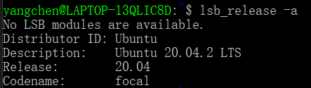
- python :3.8
2. 下载与安装
2.1 将库克隆到本地
不可直接下载,克隆该库,需要递归克隆的子模块,在需要克隆的文件夹下运行:
1 | git clone --recurse-submodules <REPOSITORY> |
该处即直接输入以下命令:
1 | git clone --recurse-submodules https://git.ist.ac.at/gsperl/HYLC.git |
2.2 安装其他依赖项
接下来使用子模块 vcpkg 安装其他依赖项:
- 先进入文件夹
vcpkg:
1 | cd vcpkg |
- 开始下载依赖库(需要科学上网):
1 | ./bootstrap-vcpkg.sh |
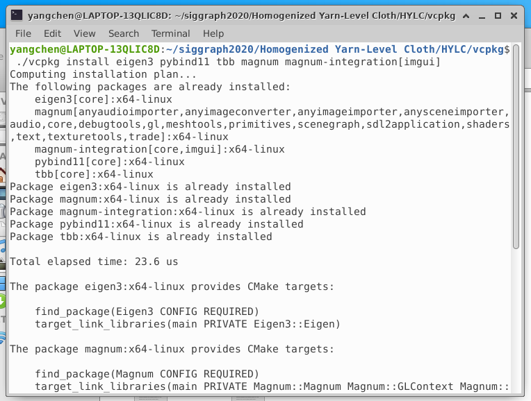
- 安装
magnum依赖项
1 | ./vcpkg install sdl2 curl |
安装完成后显示:
2.3 报错处理
2.3.1 OpenGL 相关
Could NOT find OpenGL (missing: OPENGL_opengl_LIBRARY OPENGL_glx_LIBRARY OPENGL_INCLUDE_DIR)
安装 libgl1-mesa-dev :
1 | sudo apt-get install libgl1-mesa-dev |
参考:https://stackoverflow.com/questions/31170869/cmake-could-not-find-opengl-in-ubuntu
2.3.2
Could NOT find PNG (missing: PNG_LIBRARY PNG_PNG_INCLUDE_DIR)
1 | sudo apt-get install libpng-dev |
Could NOT find GLUT (missing: GLUT_glut_LIBRARY GLUT_INCLUDE_DIR)
1 | sudo apt-get install freeglut3-dev |
1 | sudo apt-get install xorg-dev |
3. 编译运行
- 先安装 python 的一些基础库:
1 | pip3 install --user numpy scipy matplotlib |
- 进入文件夹
solver/,使用一个辅助 python 脚本进行编译和运行交互式优化可视化:
1 | python3 exec.py |
- 构建并安装 python 的相关软件包:
1 | pip3 install -e src/python/ |
- 通过 pybind11 将 c++ 模式优化暴露给 python;
- 使用
-e使其成为覆盖该软件包先前存在的安装的开发安装
4. 文件注释
Short explanation:
Using python scripts from within the ‘db2pyp.blend’ file, we load or construct periodic patterns and save them in our custom ‘.pyp’ format.
In the subdirectory DB/IDPYP we have deleted everything except a manually fixed knit pattern, as Leaf et al. did not include a license file with their data. Instead, you can just download and paste their data in there.
In the ‘db2pyp.blend’ file, you will find scripts on the right, where “load” loads a Leaf-et-al file as curves, “save” saves it as a pyp file. After loading or handcrafting a pattern you’ll have to manually set the curve objects ‘Custom Properties’ to contain a vector ‘period’ to define the periodic patch size. In between you can also look at the ‘apply’ script, that allows resampling the curves uniformly, making sure that all vertices are contained in a rectangular patch, and even tiling/repeating the pattern.
Note that we also load patterns scaled by 100 to cm units, to be better visible in blender, though we save in units of meters again. Note that Leaf et al.'s patterns might be in different scales (knit patterns usually in cm, and woven patterns smaller).
About the ‘.pyp’ format:
‘.pyp’ files and similarly the PeriodicYarnPattern (often abbreviated as PYP) class in the solver/src directory are in a self-made format for periodic yarn patterns, with all the information we found necessary to save a (rest) state. It should be somewhat documented in terms of comments in the header file of said class, and also all of the pyp files contain comments for what the blocks of data are.
E.g. the following block gives the periodic length (in m) along x and y (or also called xi0, xi1) coordinates, with a yarn radius of 0.001m. And just in case it also mentiones how many yarn segments are in this pattern. Note that due to periodicity, there are as many vertices as there are edges.
*pattern # px py radius num_vertedges
0.021428 0.01428571 0.001 251
And similarly to libWetCloths yarn model which we use for forces, almost all per-edge data is also stored as if indexed by its first vertex. As an example the 4-vectors that make up the vertex values are xyz of a vertex and the twist t(or theta) of its outgoing edge. These are stored in the *V block.
The edges *E are of the form [v0, v1, dx, dy], where v0 v1 are the incident vertex indices, and dx dy describes how many boundaries the edge crosses (which at most should be one). Edges with a nonzero dx or dy thus connect some vertex to a periodic version of it across the boundary. Having the info stored this way made it much easier for me to traverse individual periodic yarns in knits, or to tile patterns for creating ghost segments.
This is the minimum info needed to construct a periodic patch, and then after simulation it can also include information such as rest lengths, rest curvatures, discrete elastic rods reference directors, etc.
简短解释:
使用“DB2PYP.BLEND”文件中的Python脚本,我们加载或构造定期模式并以我们的自定义’.pyp’格式保存。
在子目录DB / IDPYP中,我们已删除除手动固定的针织图案之外的所有内容,如Leaf等人。没有包含其数据的许可证文件。
相反,您可以只需在那里下载并粘贴他们的数据。
在“db2pyp.blend”文件中,您将在右侧发现脚本,其中“加载”将Leaf-et-al文件加载为曲线,“保存”将其保存为PYP文件。
加载或处理模式后,您必须手动设置曲线对象’自定义属性’以包含矢量“句点”以定义周期性补丁大小。
在您之间,您也可以查看“应用”脚本,允许统一重新采样曲线,确保所有顶点都包含在矩形贴片中,甚至平铺/重复模式。
请注意,我们还将100到CM单位的加载模式加载到搅拌机中更好地可见,但我们再次以米为单位。
注意,Leaf等人。
的图案可能处于不同的尺度(通常以cm的针织图案,并且编织图案较小)。
关于’.pyp’格式:’.pyp’文件并类似地,求解器/ src目录中的句鱼纳图(通常缩写为pyp)类以自制的格式为定期纱线模式,其中我们发现的所有信息保存(休息)状态。
它应该在所述类别的标题文件中的注释方面有所记录,并且所有PYP文件也包含评论,用于数据块是什么。
例如。下面的块沿X和Y(或也称为XI0,XI1)坐标给出周期性的长度(或也称为XI0,XI1),纱线半径为0.001M。
而且,如果它还提到此模式中有多少纱线段。
请注意,由于周期性,有多个顶点,因为有边缘。
- Pattern#PX PY RADIUS NUM_VERTEDGES
0.011428 0.01428571 0.0128571 0.001 251
和与我们用于力量的Libwetcloths纱线模型,几乎所有按边级数据也被存储在其第一个顶点索引的情况下。作为一个示例,构成顶点值的4载体是顶点的XYZ和其传出边缘的扭曲T(或θ)。这些存储在* V块中。
边缘* e是形式[V0,V1,DX,Dy],其中V0 V1是入射的顶点指数,DX Dy描述了边缘交叉的边界(最多应该是一个)。
因此,具有非零DX或Dy的边缘将一些顶点连接到边界的周期性版本。具有这种方式的信息,使我更容易地遍历针织中的单个周期性纱线,或者对用于产生鬼段的瓷砖图案。
这是构建周期性补丁所需的最小信息,然后在仿真之后,它还可以包括诸如REST长度,休息曲线,离散弹性棒参考导演等信息等信息。